Michael Wrona's Blog
Engineering, coding, tech, and other cool projects!
Measuring IMU Noise Density
Sensor noise is an extremely important characteristic to consider when integrating sensors into a project. Sensor noise distorts underlying signals engineers are interested in, which makes measuring underlying processes more difficult or near impossible. Since the inertial measurement unit (IMU) is such an important system in rockets, airplanes, and satellites, not fully understanding IMU noise can be disaterous!
The first step in mitigating sensor noise is measuring and characterizing noise. Analyzing sensor noise can give you clues about what types of noise and external phenomena are distorting sensor measurements. Let’s use tape cassettes as an example. Tape hiss is the static noise you hear when no music is playing. Audio engineers can measure and characterize the tape hiss and design filters to supress hiss while simultaneously playing music.
Noise analysis is almost always performed in the frequency domain. We will convert gyro and accelerometer time-series data to the frequency domain through a Fourier transform. In this post, I’ll explain and demonstrate how to generate a frequency domain plot of both accelerometer and gyroscope data, and compute the noise spectral density - with Python code examples!
Generating the Data
Sensor noise is typically measured in situ (under normal operating conditions). For example, if we want to analyze the Boeing 737 avionics’ accelerometer noise, we’d record accelerometer data while in flight. Also, since sensor noise typically has both low and high frequency components, you should measure data at a high sample rate. For simplicity, I will measure my IMU sensor’s noise with it completely stationary at 100Hz. I recorded IMU sensor data for eight hours and logged it to a CSV file.
I used Adafruit’s Precision NXP 9-DOF IMU, which features the NXP FXOS8700 MEMS accelerometer + mangetometer and the NXP FXAS21002 MEMS gyroscope.
Load the Data File (Python)
import numpy as np
from scipy import signal
import matplotlib.pyplot as plt

DATA_FILE = 'accelgyro_still_100hz_6hrs.csv'
FS = 100  # Sample frequency [Hz]
MEAS_DUR_SEC = 28800  # (6 hrs) Seconds to record data for
TS = 1.0 / FS  # Sample period [s]

# Load into arrays, convert units
dataArr = np.genfromtxt(DATA_FILE, delimiter=',')
ax = dataArr[:, 0] * 9.80665  # m/s/s
ay = dataArr[:, 1] * 9.80665
az = dataArr[:, 2] * 9.80665
gx = dataArr[:, 3] * (180 / np.pi)  # deg/s
gy = dataArr[:, 4] * (180 / np.pi)
gz = dataArr[:, 5] * (180 / np.pi)
Standard Deviation Isn’t Sufficient
Noise standard deviation $\sigma$ or variance $\sigma^2$ is one way to quantify how noisy our sensor data is. Unfortunately, standard deviation isn’t always the best way to measure sensor noise. Some sensors downsample their data, or take the average of a few readings and output data at a lower rate. If our sensor downsamples, we cannot get an idea of the intrinsic noisiness of our sensor.
Power Spectral Density
- A power spectral density plot, or PSD plot, is a graph used to illustrate the variation of signal power with frequency. In other words, it plots signal power density as a function of frequency (source). Here’s a way I like to compare variance and power spectral density:
The variance of a signal is a time domain parameter. Power spectral density is the frequency domain counterpart of variance. Basically, power spectral density is the Fourier transform of variance (source).
A sensor’s noise spectral density is simply the power spectral density of the sensor’s noise. It is a better metric to specify sensor noise than standard deviation and is commonly used to specify IMU noise. Both the FXOS8700 and FXAS21002 datasheets specify a ’noise density’ parameter.
There are many online resources that can explain power spectral density better than I can, so I highly recommend looking it up if you’re unfamiliar.
IMU Frequency Domain (FFT) Analysis
The Fourier transform is the primary tool used to analyze noise. Fourier transforms assume that any time-series data can be decomposed into the sum of a bunch of sinusoids, each with a certain frequency and amplitude. Basically, they tell us about the frequency content of a signal and how intense the signal is at certain frequencies. The Fast Fourier Transform, or FFT, is an algorithm used to compute a Fourier transform very quickly. Again, there are plenty of resources online that can explain Fourier transfroms better than I can, so if you do not understand them, I highly reccommend looking them up.
NumPy and SciPy are fantastic Python tools for frequency domain analysis. Let’s compute and plot the Fourier transform of our gyro and accelerometer data. For simplicity, I only plotted the X-axis gyro and accelerometer data.
N = len(gx)  # Number of elements

# Compute FFTs
freqBins = np.linspace(0, FS / 2, N // 2)  # Freq. labels [Hz]
fax = np.fft.fft(ax)  # FFT of accel. data
fgx = np.fft.fft(gx)  # FFT of gyro data

# Plot x-accel. FFT
plt.figure()
plt.plot(freqBins, (2 / N) * np.abs(fax[:N // 2]))
plt.title('FFT of X-Accelerometer Data)
plt.xlabel('Frequency [Hz]')
plt.ylabel('Amplitude')
plt.grid()

# Plot x-gyro. FFT
plt.figure()
plt.plot(freqBins, (2 / N) * np.abs(fgx[:N // 2]))
plt.title('FFT of X-Gyroscope Data)
plt.xlabel('Frequency [Hz]')
plt.ylabel('Amplitude')
plt.grid()
plt.show()
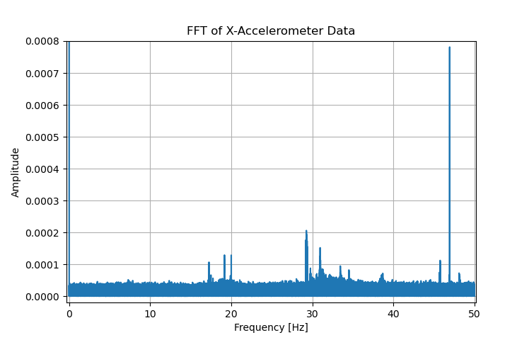
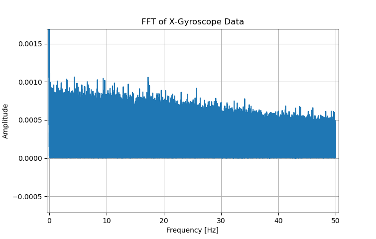
Note that the FFT only goes up to 50Hz, which is the Nyquist frequency for a sample rate of 100Hz. The gyro FFT is relatively flat, while the accelerometer FFT shows some sharp peaks. I recorded data with my IMU on a shelf below my PC. The peak at 17Hz is equal to 1020RPM, which is the average RPM of my PC’s CPU fan. I would never know that the IMU was picking up vibrations from my PC without a frequency domain plot. That is the power of Fourier transforms and frequency domain analysis! I’m still not sure what the large peak at about 47Hz is, though. It only shows up in the accelerometer data, which is kinda strange…
IMU Noise Density
Computing the noise density of our IMU data is a bit more complex. We will use SciPy’s signal.welch() function to compute the power spectral density. The signal.welch() algorithm outputs PSD in units of $(units)^2 / Hz$. On the other hand, accelerometer and gyro datasheets typically specify noise spectral density in units of $\mu g / \sqrt{Hz}$ and $dps / \sqrt{Hz}$, respectively (dps = degrees per second). Therefore, I took the square root of the signal.welch() result to compute noise density in units of $(units) / \sqrt{Hz}$,
Then, in order to compute a noise density value, we can take the average of the noise density across all frequencies.
# Conversion factor: m/s/s -> ug (micro G's)
accel2ug = 1e6 / 9.80665
# Compute PSD via Welch algorithm
freqax, psdax = signal.welch(ax, FS, nperseg=1024, scaling='density') # ax
freqay, psday = signal.welch(ay, FS, nperseg=1024, scaling='density') # ay
freqaz, psdaz = signal.welch(az, FS, nperseg=1024, scaling='density') # az
freqgx, psdgx = signal.welch(gx, FS, nperseg=1024, scaling='density') # gx
freqgy, psdgy = signal.welch(gy, FS, nperseg=1024, scaling='density') # gy
freqgz, psdgz = signal.welch(gz, FS, nperseg=1024, scaling='density') # gz
# Convert to [ug / sqrt(Hz)]
psdax = np.sqrt(psdax) * accel2ug
psday = np.sqrt(psday) * accel2ug
psdaz = np.sqrt(psdaz) * accel2ug
psdgx = np.sqrt(psdgx)
psdgy = np.sqrt(psdgy)
psdgz = np.sqrt(psdgz)
# Compute noise spectral densities
ndax = np.mean(psdax)
nday = np.mean(psday)
ndaz = np.mean(psdaz)
print('AX Noise Density: %f ug/sqrt(Hz)' % (ndax))
print('AY Noise Density: %f ug/sqrt(Hz)' % (nday))
print('AZ Noise Density: %f ug/sqrt(Hz)' % (ndaz))
ndgx = np.mean(psdgx)
ndgy = np.mean(psdgy)
ndgz = np.mean(psdgz)
print('GX Noise Density: %f dps/sqrt(Hz)' % (ndgx))
print('GY Noise Density: %f dps/sqrt(Hz)' % (ndgy))
print('GZ Noise Density: %f dps/sqrt(Hz)' % (ndgz))
# Plot accel. data
plt.figure()
plt.plot(freqax, psdax, label='ax')
plt.plot(freqay, psday, label='ay')
plt.plot(freqaz, psdaz, label='az')
plt.title('Accelerometer Power Spectral Density')
plt.xlabel('Frequency [Hz]')
plt.ylabel(r'Spectral Density $\mu g / \sqrt{Hz}$')
plt.legend()
plt.grid()
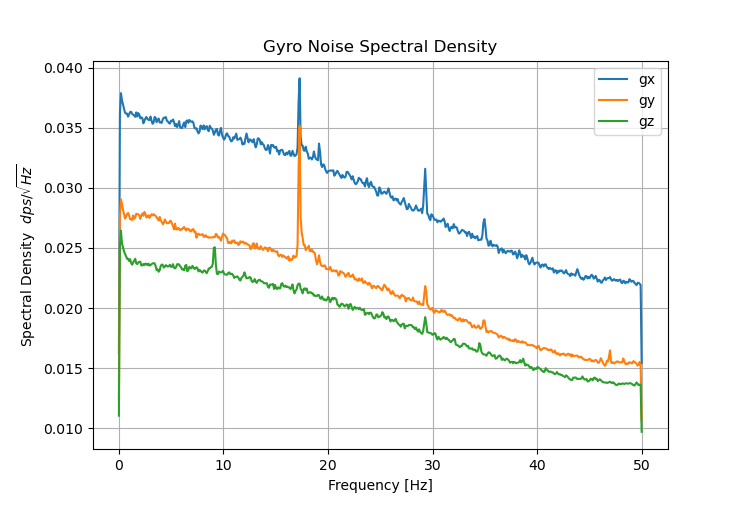
# Plot gyro data
plt.figure()
plt.plot(freqgx, psdgx, label='gx')
plt.plot(freqgy, psdgy, label='gy')
plt.plot(freqgz, psdgz, label='gz')
plt.title('Gyro Noise Spectral Density')
plt.xlabel('Frequency [Hz]')
plt.ylabel(r'Spectral Density $dps / \sqrt{Hz}$')
plt.legend()
plt.grid()
plt.show()
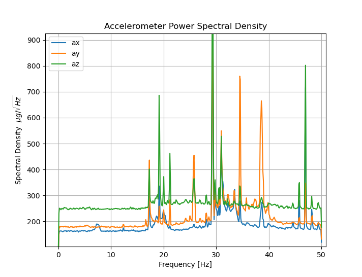
FXOS8700 Accelerometer
| Accelerometer Axis | Noise Density $\mu g / \sqrt{Hz}$ |
|---|---|
| AX | 191.982827 |
| AY | 221.099756 |
| AZ | 272.502801 |
The FXOS8700 datasheet specified a noise density of 126 $\mu g / \sqrt{Hz}$, which is a bit off from our measurements. This is likely due to the sharp peaks in the accelerometer data. If we computed the average without including the peaks, I’m sure it would be closer to the datasheet value.
FXAS21002 Gyroscope
| Gyroscope Axis | Noise Density $dps / \sqrt{Hz}$ |
|---|---|
| GX | 0.029333 |
| GY | 0.021520 |
| GZ | 0.019020 |
The FXAS21002 datasheet specified a noise density of 0.025 $dps / \sqrt{Hz}$, which is very close to our measurements.