Michael Wrona's Blog
Engineering, coding, tech, and other cool projects!
Gyro Noise and Allan Deviation + IMU Example
Rate gyros measure angular rotation rate, or angular velocity, in units of degrees per second [deg/s] or radians per second [rad/s]. Gyros are used across many diverse applications. Since I come from an aerospace background, I know that gyros are extremely important sensors in rockets, satellies, missiles, and airplane autopilots.
When SpaceX and Rocket Lab designed control systems for their rockets, they invested a significant amount of time and resources into creating very accurate vehicle simulations. One aspect of creating their simulation involved modelling the sensors engineers planned on incorporating into their final control systems. Properly modelling sensors enabled engineers to analyze how well the system performed with different sensor configurations and determined the best one.
Since gyros are arguably the most important sensors in a control system, a proper gyro model is a significant contributor towards achieving an accurate vehicle simulation. And in order to model a gyro sensor, we need to characterize its noise!
In this article, I’ll explain the two most important gyro noise characteristics and how to determine them from an Allan deviation plot (with code, too). I’ll also compute the Allan deviation and noise characteristics of the NXP FXAS21002 3-DOF gyro.
Gyro Noise Parameters
In my opinion, the two most important gyro noise characteristics to consider are:
- Angle Random Walk (unit:
$\deg / \sqrt{hr}$) - Bias Instability (unit:
$\deg / hr$)
There are other noise parameters that one can determine, but in my opinion, these are the two most important.
Angle Random Walk (ARW)
- Random walk is a mathematical model used to describe a random process that consists of a random succession of steps, typically applied to time-series data. The analogy that I like to use is as follows:
Let’s say you’re standing on the 50 yard line of a football field with a coin. If you flip heads, you move forward one step, and if you flip tails, you move back one step. Do this 100 times. You’ll either end up forwards or backwards of your starting point. You had equal probability of moving forwards or backwards at each coin flip. If you were to restart on the 50 yard line and repeat the 100 coin flips many times, you’d end in a different location every time. This is the nature of a random walk process!
Here’s how random walk relates to gyros. Gyro rate measurements are typically time-integrated to compute angles. This integration will drift over time due to sensor noise. This drift appears as the integrated gyro angle taking random steps from sample to sample, hence the term gyro ANGLE random walk (ARW).
The unit for angle random walk is typically $deg / \sqrt{hr}$, but is sometimes given in $deg / \sqrt{sec}$. If we multiply the angle random walk by the square root of time, the standard deviation $\sigma$ of drift due to noise can be computed. Therefore, angle measurements from a gyro with low ARW will not drift much over time due to random noise. Angle measurements from a gyro with high ARW will drift more due to random noise with a higher deviation. Cheap MEMS gyros, like the MPU6050 and BNO055, will have higher ARW compared to fancy (and very expensive) laser or fiber optic gyros.
Bias Instability
In my opinion, gyro bias instability is the most important charactersitic to consider when comparing gyro sensors. All gyro sensors, regardless of price or quality, will have measurement biases. Measurement bias is a constant measurement offset from true. Gyro biases will cause angle drift in time-integrated data. For example, When the gyro is switched on and remains stationary, the sensor will read a slight non-zero rate measurement. This bias is called turn-on bias.
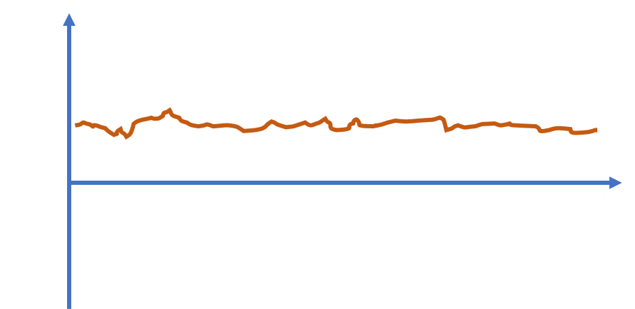
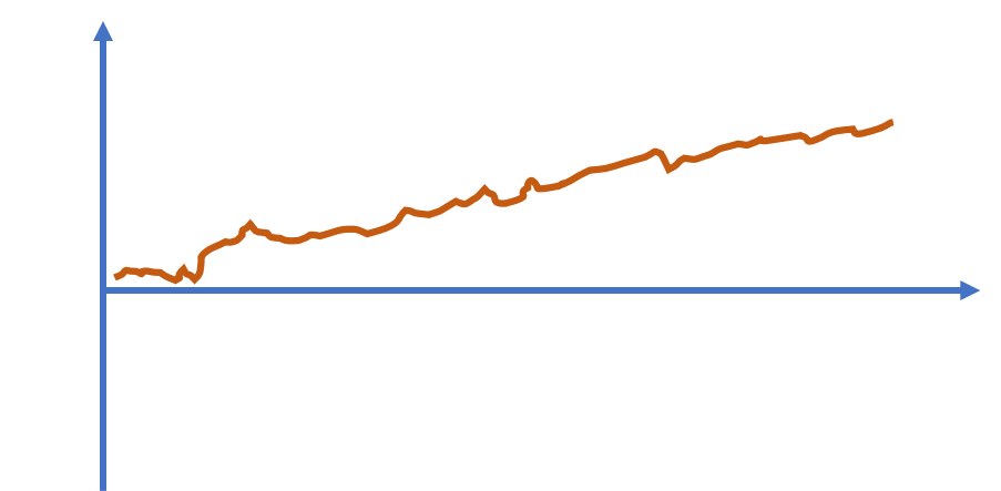
In reality, gyro bias is not constant - it gradually changes over time. Gyro bias instability is a measure of how much gyro biases drift over time. Gyro bias instability is typically given in units of $deg / hr$. Low bias instability means that gyro biases are relatively stable and don’t change much. High bias instability means that gyro biases are less stable and change quicker.
Another way to illustrate the importance of gyro bias instability is from a sensor fusion/state estimation perspective. State estimation algorithms (such as Kalman Filters) that fuse gyro, accelerometer, and GPS data will typically estimate gyro biases. These estimation algorithms commonly assume gyro biases are constant. If the gyro sensor bias instability is high, the bias will drift and the estimation algorithms will have a difficult time estimating biases.
Allan Deviation
Allan variance was originally derived to measure the noise characteristics and stability of clock oscillators. More specifically, the frequency stability of oscillators. Allan variance analyses are used to estimate the stability of a time-domain signal due to noise processes, not systematic errors such as temperature effects. I should note Allan deviation is simply the square root of Allan variance, i.e.
$$Deviation = \sqrt{Variance}$$
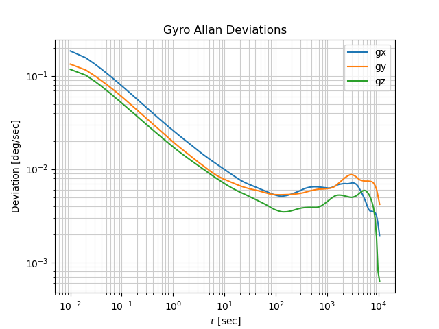
Allan deviation can also be applied to analyze the stability and noise characteristics of gyro sensors. We will compute the Allan deviation of gyro angle data in degrees. The result of an Allan deviation analysis is a plot, typically plotted on a log scale. The x-axis will be time in seconds, and the y-axis will be Allan deviation in degrees per second.
Noise Analysis Example
I will be analyzing the FXAS21002 MEMS gyro sensor within Adafruit’s NXP Precision 9-DOF IMU. First, I’ll explain the data collection process. Then, I’ll walk you through my code to compute the Allan deviation. Finally, I’ll demonstrate how to compute the angle random walk and bias instability of our gyro sensor from an Allan deviation plot.
Data Collection
Since we are measuring the long-term stability of a gyro, we will need to collect data for a long time. I recorded stationary gyro data at 100Hz for 6 hours. I wrote some Arduino code to read the I2C sensor and print data over a serial connection so that my computer could read and write it to a CSV file.
Arduino Code (C++, Simplified)
....
....

void loop()
{
    now = millis();

    if (now - then >= 10)
    {
        // Data in [rad/s]
        Serial.print(Gyro.GetGx(), 6); Serial.print(",");
        Serial.print(Gyro.GetGy(), 6); Serial.print(",");
        Serial.println(Gyro.GetGz(), 6);
        then = now;
    }
}
Data Logging Code (Python)
import csv
import serial

SERIAL_PORT = 'COM10'
SERIAL_BAUD = 115200
OUT_FILE = 'gyro-data.csv'
FS = 100  # Sample frequency [Hz]
MEAS_DUR_SEC = 21600  # (6 hrs) Seconds to record data for

TS = 1.0 / FS  # Sample period [s]
N_SAMPLES = int(MEAS_DUR_SEC * FS)  # Number of samples to record

# Init. serial
ser = serial.Serial(SERIAL_PORT, SERIAL_BAUD)
ser.flush()

with open(OUT_FILE, newline='', mode='w') as csvfile:
    csvwriter = csv.writer(csvfile, delimiter=',')

    for _ in range(N_SAMPLES):
        # Read serial stream and extract data
        dataList = ser.readline().decode('utf-8').strip('\r\n').split(',')

        # Write data to CSV file: gx,gy,gz
        csvwriter.writerow(dataList)
Allan Deviation Computation
We will be computing the Allan deviation of gyro angle data in degrees. First, I imported the gyro rate data into numpy arrays. Then, I converted the raw gyro rate data from $rad/s$ to $deg/s$. Next, I Euler integrated the rate data to compute gyro orientation data in $deg$ by computing the cumulative sum (numpy.cumsum()) of the data and multiplying it by the sample period (0.01sec). I then passed the gyro angle data to my Allan deviation function and computed the Allan variance in $deg/s$. Finally, I plotted the data on a log-scale plot.
Allan Variance Code (Python)
import numpy as np
import matplotlib.pyplot as plt


# Config. params
DATA_FILE = 'gyro-data.csv'  # CSV data file "gx,gy,gz"
fs = 100  # Sample rate [Hz]

def AllanDeviation(dataArr, fs, maxNumM=100):
    ....

# Load CSV into np array
dataArr = np.genfromtxt(DATA_FILE, delimiter=',')
ts = 1.0 / fs

# Separate into arrays
gx = dataArr[:, 0] * (180.0 / np.pi)  # [deg/s]
gy = dataArr[:, 1] * (180.0 / np.pi)
gz = dataArr[:, 2] * (180.0 / np.pi)

# Calculate gyro angles
thetax = np.cumsum(gx) * ts  # [deg]
thetay = np.cumsum(gy) * ts
thetaz = np.cumsum(gz) * ts

# Compute Allan deviations
(taux, adx) = AllanDeviation(thetax, fs, maxNumM=200)
(tauy, ady) = AllanDeviation(thetay, fs, maxNumM=200)
(tauz, adz) = AllanDeviation(thetaz, fs, maxNumM=200)

# Plot data on log-scale
plt.figure()
plt.title('Gyro Allan Deviations')
plt.plot(taux, adx, label='gx')
plt.plot(tauy, ady, label='gy')
plt.plot(tauz, adz, label='gz')
plt.xlabel(r'$\tau$ [sec]')
plt.ylabel('Deviation [deg/sec]')
plt.grid(True, which="both", ls="-", color='0.65')
plt.legend()
plt.xscale('log')
plt.yscale('log')
plt.show()
Allan Deviation Algorithm (Python)
import numpy as np

def AllanDeviation(dataArr: np.ndarray, fs: float, maxNumM: int=100):
    """Compute the Allan deviation (sigma) of time-series data.

    Algorithm obtained from Mathworks:
    https://www.mathworks.com/help/fusion/ug/inertial-sensor-noise-analysis-using-allan-variance.html

    Args
    ----
        dataArr: 1D data array
        fs: Data sample frequency in Hz
        maxNumM: Number of output points

    Returns
    -------
        (taus, allanDev): Tuple of results
        taus (numpy.ndarray): Array of tau values
        allanDev (numpy.ndarray): Array of computed Allan deviations
    """
    ts = 1.0 / fs
    N = len(dataArr)
    Mmax = 2**np.floor(np.log2(N / 2))
    M = np.logspace(np.log10(1), np.log10(Mmax), num=maxNumM)
    M = np.ceil(M)  # Round up to integer
    M = np.unique(M)  # Remove duplicates
    taus = M * ts  # Compute 'cluster durations' tau

    # Compute Allan variance
    allanVar = np.zeros(len(M))
    for i, mi in enumerate(M):
        twoMi = int(2 * mi)
        mi = int(mi)
        allanVar[i] = np.sum(
            (dataArr[twoMi:N] - (2.0 * dataArr[mi:N-mi]) + dataArr[0:N-twoMi])**2
        )

    allanVar /= (2.0 * taus**2) * (N - (2.0 * M))
    return (taus, np.sqrt(allanVar))  # Return deviation (dev = sqrt(var))
Interpreting Allan Deviation Plots
Allan deviation plots are always given on a log scale plot (X and Y axes are log-scale). The X-axis is typically in units of seconds or hours, and the Y-axis Allan deviation in units of $deg/hr$ or $deg/sec$. Our code’s plot is in units of seconds and $deg/sec$. I’ll use the X-gyro (gx) data for example calculations.
Gaussian White Noise
We can determine if our gyro has Guassian white noise from an Allan deviation plot. If it does, then the slope of the Allan deviation plot on the left side should be -0.5. I fit a curve with a slope of -0.5 to our X-gyro data and got this plot:
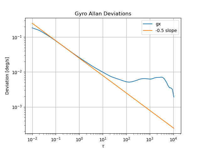
The -0.5 slope line matches well with our plot. Therefore, our sensor has Guassian white noise. This is important to verify, because most sensor fusion algorithms, such as Kalman Filters, assume state observations (measurements) have Gaussian white noise.
Angle Random Walk
First, determine the Allan deviation at $\tau = 1s = 10^{0}s$. For my X-gyro data, the Allan deviation is about $0.026 deg/s$. Then, we multiply this by 60 to get angle random walk in $deg / \sqrt{hr}$.
$$ ARW = 0.026 \frac{deg}{s} * 60 \frac{s}{\sqrt{hr}} $$
$$ ARW = 1.56 \frac{deg}{\sqrt{hr}} $$
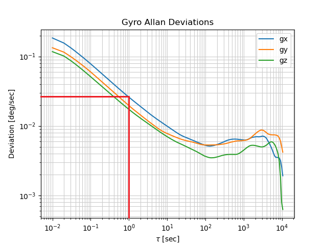
Therefore, our X-gyro angle random walk is $1.56 deg/\sqrt{hr}$.
Bias Instability
Computing bias instability is a bit trickier. As we can see in the Allan deviation plot, the data reaches a minimum before increasing again. First, determine the Allan deviation at this minimum point in $deg/s$. For my X-gyro data, this point was at $\tau=129.1s$ and the deviation was $0.005 deg/s$. Then, we divide this value by 0.664 and multiply the result by 3600. This yields bias instability in $deg/hr$. The 0.664 is a dimensionless value specified in IEEE Standard 952-1997 and is a constant in some icky math equation.
$$ BI = 0.005 \frac{deg}{s} * \frac{1}{0.664} * 3600\frac{s}{hr} $$
$$ BI = 27.1 deg / hr $$
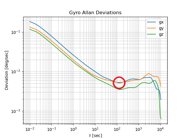
Therefore, our X-gyro bias instability is $27.1 deg / hr$.
Conclusion
| FXAS21002 X-Gyro Noise Data | |
|---|---|
| Angle Random Walk | $1.56 deg / \sqrt{hr}$ |
| Bias Instability | $27.1 deg / hr $ |
Measuring the noise of gyroscope sensors is a very important step in sensor modelling. Having accurate sensor models will directly influence and significantly affect how accurate a simulation will be. Two very important gyro noise characteristics are angle random walk and bias instability. Allan deviation analyses can be used to determine these characteristics from stationary gyro angle measurements. Both characteristics can be easily interpreted from an Allan deviation plot.
Thanks so much for reading!