Introduction

The first few algorithms introduced in numerical methods courses are typically root-finding algorithms. In my opinion, these algorithms are taught first because they are relatively easy to understand and code, and determining roots of a function is a very common math operation. They also introduce fundamental numerical analysis topics, such as convergence criteria and iterative operations.

A root, or zero, of a function $f$ is a point $x_0$ that satisfies $f(x_0) = 0$. An arbitrary function may have multiple roots. The Bisection Method is one of the most utilized root-finding algorithms due to its simplicity. Note that the Bisection Method is also sometimes referred to as the Binary-Search Method. The Bisection Method is derived from the Intermediate Value Theorem. In this context, the Intermediate Value Theorem is defined as:

For some function $f(x)$ that is defined on the interval $[a, b]$, if the sign of $f(a)$ and $f(b)$ is opposite, there must exist a value $p$ such that $f(p) = 0$.

I’ll translate this definition into something more general. Root-finding numerical methods typically accept a function and boundary points (x-values) where we believe a root lies. The lower(left) bound is $x = a$ and the upper (right) bound is $x = b$. First, we need to make sure our function $f(x)$ is continuous and exists between our boundaries $[a, b]$. An easy way to verify this is to plot the function. Next, we evaluate our function at $x = a$ and $x = b$, i.e. determine $f(a)$ and $f(b)$. If the signs of $f(a)$ and $f(b)$ differ, the function must have crossed zero at some point within $[a, b]$. This means that there must be some point $x = p$ where the function crossed the x-axis, or in other words, make $f(p) = 0$ - a root!

The Bisection Method

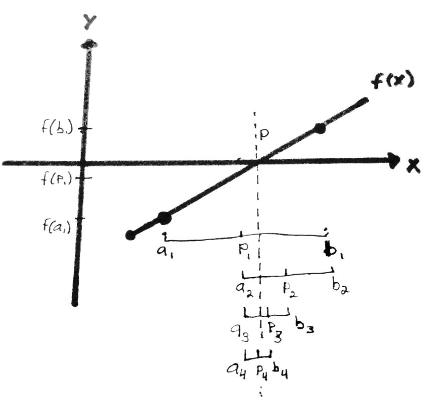
Next, I’ll explain how the Bisection Method determines roots. The first step is choosing initial $a$ and $b$ boundary values that we believe the root is within. Let’s call these $a_1$ and $b_1$. Next, we determine the midpoint $p_1$ between $a$ and $b$ via:

$$p_1 = a_1 + \frac{b_1 - a_1}{2} = \frac{a_1 + b_1}{2}$$

Then, the boundary points $a$ and $b$ and the computed midpoint $p$ can be compared:

• If $f(p_1)$ and $f(a_1)$ have the same sign, $p$ must exist between $p_1$ and $b_1$.
• If $f(p_1)$ and $f(a_1)$ have opposite signs, $p$ must exist between $a_1$ and $p_1$.

This relationship can be seen in Figure 1. Since $f(p_1)$ and $f(a_1)$ have the same sign in Figure 1, the root must lie between $p_1$ and $b_1$. Then, we can update the new interval to be $p_1$ and $b_1$. Therefore, we can set $a_2 = p_1$ and $b_2 = b_1$. Then, using the above equation, a new midpoint $p_2$ can be computed. The sign check is performed again, and a new interval is determined. This continues until the interval becomes sufficiently small, with the root approximation at the midpoint of the small interval.

Bisection Method Steps

The steps for the Bisection Method looks something like:

• Choose initial boundary points $a_1$ and $b_1$.
• Compute the midpoint $p_1 = \frac{a_1 + b_1}{2}$.
• Determine the new interval:
  • If $f(p_1)$ and $f(a_1)$ have the same sign, set $a_2 = p_1$ and $b_2 = b_1$.
  • If $f(p_1)$ and $f(a_1)$ have opposite signs, set $a_2 = a_1$ and $b_2 = p_1$.
• Repeat until interval $[a_n, b_n]$ becomes sufficiently small.

Pros and Cons

Advantages

• Easy to understand conceptually.
• Easy to implement in code.
• Always will converge to a solution, but not necessarily the correct one.

Drawbacks

• Relatively slow to converge compared to other methods (takes more iterations).
• Doesn’t work well when the root is located where the function is flat (near-zero slope).
• Convergence speed depends on how ‘wide’ the initial interval is (smaller = faster).

Convergence Check

As the Bisection Method converges to a zero, the interval $[a_n, b_n]$ will become smaller. To check if the Bisection Method converged to a small interval width, the following inequality should be true:

$$\frac{b - a}{2} < \epsilon$$

The Greek letter epsilon, $\epsilon$, is commonly used to denote tolerance. In code, I like to use the variable name TOL. The above convergence check is very easy to implement and works just fine. Another way to check convergence is by computing the change in the value of $p$ between the current ($i$) and prevoius ($i-1$) iteration.

$$\frac{|p_i - p_{i-1}|}{p_i} < \epsilon$$

Both ways work fine, but I personally prefer to use the second method, as it is a convergence criteria for many other numerical methods.

Code Implementation (Python)

So, now that we understand how the Bisection Method works, let’s code it. We will try to find a value of $x$ that solves:

$$xe^{2x} - \sqrt{x} = 4x$$

We can rearrange the equation such that one side of the equation is equal to zero:

$$f(x) = xe^{2x} - \sqrt{x} - 4x = 0$$

Let’s define this in Python code:

import numpy as np
import matplotlib.pyplot as plt

def funct(x):
    fx = (x * np.exp(2 * x)) - np.sqrt(x) - (4 * x)
    return fx

Upon inspection of $f(x)$, one solution/root of the equation is $x = 0$. This is a trivial solution, however. Let’s plot it to determine where the other solution/root is.

x_points = np.linspace(0, 1, 80)  # Points to pass to function

plt.figure()  # Plot f(x)
plt.plot(x_points, funct(x_points))
plt.title(r'$f(x) = xe^{2x} - \sqrt{x} - 4x$')
plt.xlabel('x')
plt.ylabel('f(x)')
plt.grid()

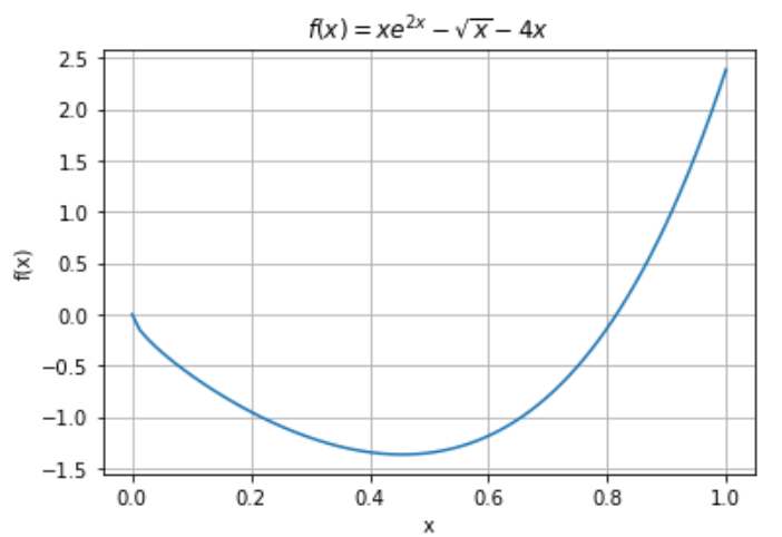
As we can see, the other solution is between $x = 0.6$ and $x = 1.0$. We’ll use these as our initial boundary points: $a_1 = 0.6$ and $b_1 = 1.0$. We can choose a tolerance value of $\epsilon = 10^{-6}$ and limit the number of iterations to 500. Here is the code for the Bisection Method:

# Initial bounds where we believe the solution/root is.
a = 0.6  # Left boundary
b = 1.0  # Right boundary

TOL = 1e-6      # Relative tolerance convergence criteria
MAX_ITER = 500  # Max. number of iterations

p_prev = 0.0    # Keep track of old p-values
soln = 0.0      # Store final solution in this variable
f_a = funct(a)  # Evaluate left point
for iters in range(MAX_ITER):   # Iterate until max. iterations are reached.
    
    p = a + ((b - a) / 2.0)     # Determine center of the interval, p
    f_p = funct(p)              # Evaluate midpoint 

    # Check if tolerance is satisfied
    if f_p == 0.0 or np.abs(p - p_prev) / np.abs(p) < TOL:
        # Break if tolerance is met, return answer!
        soln = p
        break
    
    # Determine new bounds depending on the values of f(a) and f(p)
    if (np.sign(f_a) * np.sign(f_p)) > 0.0:
        a = p       # If positive, move to the left
        f_a = f_p
    else:
        b = p       # Otherwise (if negative), move to the right

    p_prev = p      # Replace old with new


# PRINT RESULTS!
print("Bisection Method Results:")
print("    Final Tolerance: %g" % (np.abs(p - p_prev) / np.abs(p)))
print("    Number of Iterations: %g" % (iters))
print("    Solution: x = %g" % (soln))

Bisection Method Results:
    Final Tolerance: 9.35719e-07
    Number of Iterations: 18
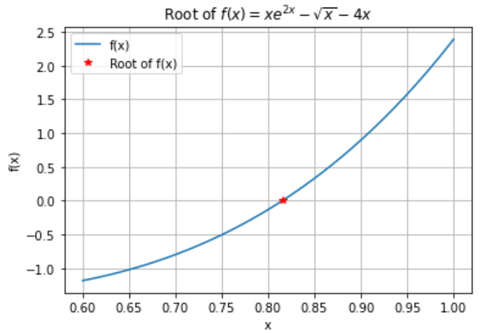
    Solution: x = 0.815351

Therefore, $x = 0.815351$ satisfies the equality $xe^{2x} - \sqrt{x} = 4x$. We can plot this point over top of the plot of $f(x) = xe^{2x} - \sqrt{x} - 4x$ to verify our solution.

x_points = np.linspace(0.6, 1.0, 80)

plt.figure()  # Plot f(x)
plt.plot(x_points, funct(x_points), label='f(x)')
plt.plot(soln, funct(soln), 'r*', label='Root of f(x)')
plt.title(r'Root of $f(x) = xe^{2x} - \sqrt{x} - 4x$')
plt.xlabel('x')
plt.ylabel('f(x)')
plt.legend()
plt.grid()

Bisection Method Python Function

Finally, here is a pretty good Python implementation of the Bisection Method:

import numpy as np


def BisectionMethod(
    a0: float,
    b0: float,
    funct,
    TOL:float=1e-6,
    MAX_ITER:int=500) -> float:
    """Solve for a function's root via the Bisection Method.

    Args
    ----
        a0: Initial left boundary point
        b0: Initial right boundary point
        funct (function): Function of interest, f(x)
        TOL: Solution tolerance
        MAX_ITER: Maximum number of iterations
    
    Returns
    -------
        p: Root of f(x) within [a, b]
    """
    p_prev = 0.0    # Keep track of old p-values
    soln = 0.0      # Store final solution in this variable
    f_a = funct(a)  # Evaluate left point
    for iters in range(MAX_ITER):   # Iterate until max. iterations are reached.
        p = a + ((b - a) / 2.0)     # Determine center of the interval, p
        f_p = funct(p)              # Evaluate midpoint 

        # Check if tolerance is satisfied
        if f_p == 0.0 or np.abs(p - p_prev) / np.abs(p) < TOL:
            # Break if tolerance is met, return answer!
            soln = p
            break
        
        # Determine new bounds depending on the values of f(a) and f(p)
        if (np.sign(f_a) * np.sign(f_p)) > 0.0:
            a = p       # If positive, move to the left
            f_a = f_p
        else:
            b = p       # Otherwise (if negative), move to the right

        p_prev = p      # Replace old with new
    
    return p

# Replace with your own function
def MyFunction(x):
    return x - 2.0


# Initial bounds where we believe the solution/root is.
a = 1.0  # Left boundary
b = 4.0  # Right boundary

root = BisectionMethod(a, b, MyFunction)
print("Root x = ", root)