One of the most important parts of any aerospace control system are the sensor fusion and state estimation algorithms. This software system is responsible for recording sensor observations and ‘fusing’ measurements to estimate parameters such as orientation, position, and speed. The quality of sensor fusion algorithms will directly influence how well your control system will perform. Poor, low-grade sensor fusion software will result in poor controller performance. Therefore, especially for costly aerospace systems, designing robust, efficient, and high-performance sensor fusion software is extremely important to ensuring mission success. One of the most popular sensor fusion algorithms is the Extended Kalman Filter (EKF). Unlike the linear Kalman Filter, EKFs are nonlinear and can therefore more accurately account for nonlinearities in sensor measurements and system dynamics. One popular sensor fusion application is fusing inertial measurement unit (IMU) measurements to estimate roll, pitch, and yaw/heading angles. This article will describe how to design an Extended Kalman Filter (EFK) to estimate NED quaternion orientation and gyro biases from 9-DOF (degree of freedom) IMU accelerometer, gyroscope, and magnetomoeter measurements.

Background

Coordinate System

Orientation needs to be defined relative to something. We will be resolving orientation relative to the NED (North, East, Down) reference frame. In the NED frame, the positive X-axis points towards true north, the positive Z-axis is parallel to gravitational acceleration downwards, and the Y-axis completes the right-handed triad.

Quaternions

We will be using quaternions to describe our IMU’s orientation. Quaternions (denoted as $q$) are a four-parameter set used to describe orientation. Compared to Euler angles, quaternions do not suffer from gimbal lock and are more numerically stable and computationally efficient. Quaternion orientation is described as a rotation angle $\theta$ about an Euler axis $\vec{e}$.

$$\begin{equation} \vec{q} = \begin{bmatrix} q_0 \\ q_1 \\ q_2 \\ q_3 \end{bmatrix} = \begin{bmatrix} cos\theta \\ e_1 sin(\theta/2) \\ e_2 sin(\theta/2) \\ e_3 sin(\theta/2) \end{bmatrix} \end{equation}$$

The quaternion kinematic differential equation is given in equation $\eqref{eq:quat-kin}$ in matrix form, and relates body angular velocities to quaternions:

$$ \begin{equation} \begin{bmatrix} \dot{q_0} \\ \dot{q_1} \\ \dot{q_2} \\ \dot{q_3} \end{bmatrix} = \frac{1}{2} \begin {bmatrix} -q_1 & -q_2 & -q_3 \\ q_0 & -q_3 & q_2 \\ q_3 & q_0 & -q_1 \\ -q_2 & q_1 & q_0 \end{bmatrix} \begin{bmatrix} \omega_1 \\ \omega_2 \\ \omega_3 \end{bmatrix} \label{eq:quat-kin} \end{equation}$$

Euler Angles and Quaternions

Euler angles are a three-parameter set used to describe orientation. In particular, we will be using the ‘3-2-1’ Euler angles, commonly referred to as roll ($\phi$), pitch ($\theta$), and yaw (or heading) ($\psi$), respectively. Euler angles are intuitive and easy to visualize, but suffer from gimbal lock when pitch angle $\theta$ is 90 degrees, and have a trigonometric kinematic relationship, which is more computationally complex. We can use equations $\eqref{eq:quat2roll}$ through $\eqref{eq:quat2yaw}$ to convert from quaternions to Euler angles.

$$\begin{equation} \phi = atan2 \left( 2(q_2 q_3 + q_0 q_1), \quad q_0^2 - q_1^2 - q_2^2 + q_3^2 \right) \label{eq:quat2roll} \end{equation}$$ $$\begin{equation} \theta = -asin \left( 2(q_1 q_3 - q_0 q_2) \right) \label{eq:quat2pitch} \end{equation}$$ $$\begin{equation} \psi = atan2 \left( 2(q_1 q_2 + q_0 q_3), \quad q_0^2 + q_1^2 - q_2^2 - q_3^2 \right) \label{eq:quat2yaw} \end{equation}$$

Gyroscope Measurement Model

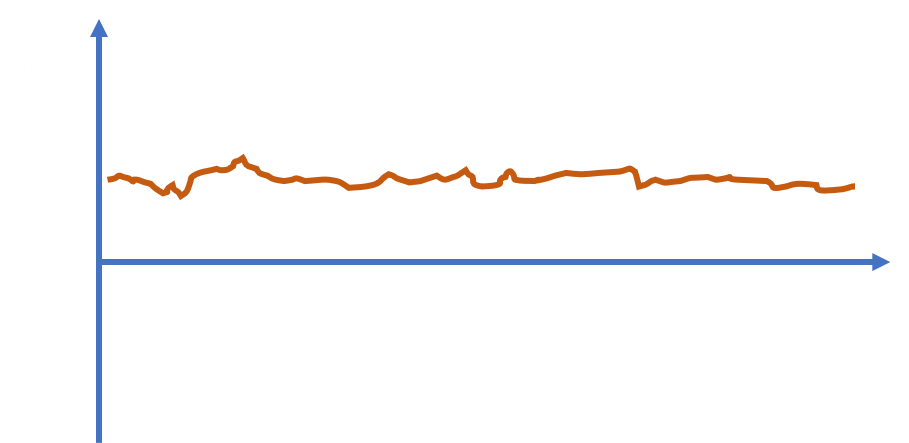
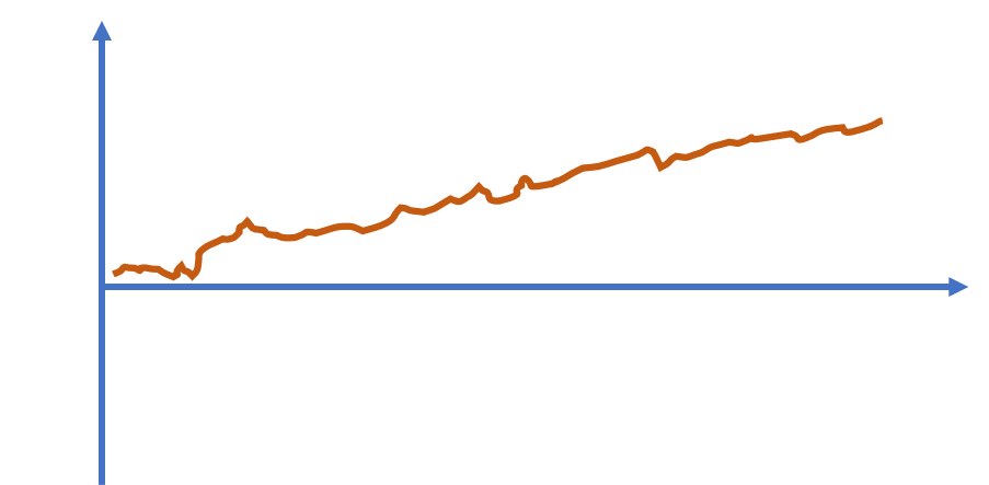
Gyroscopes measure body angular rotation rates in degrees per second [deg/s]. Ideally, gyro measurements could be time-integrated to compute body angles in degrees. Unfortunately, this direct integration is not possible due to gyro offset and gyro drift. If raw gyro measurements were taken while stationary, the readings would be close to zero, but non-zero. This offset from zero while stationary is called gyro offset or gyro bias. If these raw gyro measurements were time-integrated, the computed angles would slowly increase over time, despite the gyro being stationary. This angle ‘drift’ is called gyro drift. Therefore, gyro measurement offset causes gyro drift in time-integrated gyro measurements. An illustration of gyro drift can be seen below.

Gyro bias can be determined experimentally and hard-coded into software. This is the simplest approach and may suffice for recreational applications. However, it is very advantageous and relatively simple to estimate gyro bias with an EKF. In order to estimate gyro bias, a measurement model must be developed. It is assumed that gyro bias is time-invariant, or constant with time, in this derivation. In reality, the gyro bias varies with time and temperature, but the change is typically small, making constant bias a reasonable simplification. Equation $\eqref{eq:gyro-model}$ is the simplified sensor model used in this derivation.

$$\begin{equation} \vec{\omega}_{corr} = \vec{\omega}_{meas} - \vec{b} \quad , \quad \dot{b} = 0 \label{eq:gyro-model} \end{equation}$$

Where $\vec{\omega}_{corr}$ are the corrected gyro measurements (three measurements), $\vec{\omega}_{meas}$ are the measured gyro readings, and $\vec{b}$ are the gyro biases to be estimated.

Roll and Pitch From Accelerometer Measurements

One important operation performed in our EKF will be computing roll and pitch angles from accelerometer measurements. Since we assume gravitational acceleration is straight down in our coordinate system, we can compute roll and pitch angles relative to the gravity vector. A detailed derivation of this method can be found here. We will assume the positive Z-axis is parallel to gravitational acceleration downwards, and the XY plane is perpendicular to gravity. Since gravity is independent of heading angle, yaw angle cannot be determined from accelerometer measurements. To put it simply, we cannot measure heading with an accelerometer and gyro because gravity does not depend on heading. The equations to compute roll and pitch from accelerometer measurements are given in equations $\eqref{eq:accel2roll}$ and $\eqref{eq:accel2pitch}$.

$$\begin{equation} Roll = \phi = arctan \frac{a_y}{a_z} \label{eq:accel2roll} \end{equation}$$ $$\begin{equation} Pitch = \theta = arcsin \frac{a_x}{g} = arcsin \frac{a_x}{\sqrt{a_x^2 + a_y^2 + a_z^2}} \label{eq:accel2pitch} \end{equation}$$

Where $a_x, a_y$ and $a_z$ are the accelerometer measurements. It is important to note that these equations are valid only when the accelerometer is stationary and not influenced by accelerations other than gravitational. These equations should still work for most applications, accept dynamic ones.

Tilt-Compensated Compass

Three-axis magnetometers are essentially three-dimensional compasses. They measure the local magnetic field vector, including earth’s magnetic field. External paramagnetic and electromagnetic sources can cause hard and soft-iron distortions to magnetometer measurements. These distortions can be accounted for through calibration. We will assume that the magnetometer measurements are already calibrated for hard and soft-iron distortions.

Also, the NED coordinate frame is relative to true north. Our magnetometer measures earth’s magnetic field and therefore compass heading relative to magnetic north. The difference in heading between true north and magnetic north is called magnetic declination, often denoted as $\delta$. Magnetic declination is dependent on latitude, longitude, and altitude. Declination, field strength, and other parameters can be determined via an earth magnetic field model, such as the World Magnetic Model 2020 (WMM2020).

In order to compute true heading from magnetometer measurements and correct for sensor tilt, we will create a ’tilt-compensated compass’ using equation $\eqref{eq:tilt-compass}$.

$$\psi_{true} = \psi_{mag} + \delta $$

$$\begin{equation} \psi_{true} = atan2 \begin{pmatrix} -m_y cos\phi + m_z sin \phi \\ m_x cos\theta + m_y sin\phi sin\theta + m_z cos\phi sin\theta \end{pmatrix} + \delta \label{eq:tilt-compass} \end{equation}$$

Where $\psi_{true}$ is true heading, $\psi_{mag}$ is magnetic heading, and $m_x$, $m_y$, and $m_z$ are (calibrated) magnetometer measurements. Roll and pitch can be determined from accelerometer measurements and used in equation $\eqref{eq:tilt-compass}$.

EKF Development

All Kalman filters have two main steps - a prediction step and an update step. For our EKF prediction step, gyroscope measurements will be recorded at a high sample rate and used to estimate/predict state variables between accelerometer and magnetometer updates. The EKF update step will use lower-rate accelerometer and magnetometer measurements to correct and update state variables. State variables, EKF equations, transition equations, and measurement models will be discussed in the next sections.

State Variables

As previously mentioned, we are interested in designing an EKF to estimate quaternion orientation and gyro biases from accelerometer, gyroscope, and magnetometer measurements. The state variables we will estimate with our EKF will be the four quaternion parameters and three gyro biases, for a total of seven state variables. The state vector is given in equation $\eqref{eq:state-vec}$.

$$\begin{equation} \vec{x} = \begin{bmatrix} q_0 & q_1 & q_2 & q_3 & b_x & b_y & b_z \end{bmatrix} \label{eq:state-vec} \end{equation}$$

Prediction Step & Transition Equations

The prediction step of our EKF will use gyro measurements to estimate and ‘propagate’ state variables between accelerometer and magnetometer measurements. The quaternion differential equation given in equation $\eqref{eq:quat-kin}$ and the gyro measurement model in equation $\eqref{eq:gyro-model}$ will be time integrated and propagated to estimate state variables. The prediction step in EKFs are given in equations $\eqref{eq:ekf-pred1}$ through $\eqref{eq:ekf-pred3}$. More information about the Kalman Filter and EKF equations can be readily found online.

$$\begin{equation} \hat{x}_k^{-} = f(\hat{x}_{k-1}) \label{eq:ekf-pred1} \end{equation}$$ $$\begin{equation} P_k^{-} = F_k P_{k-1} F_k^T + Q \label{eq:ekf-pred2} \end{equation}$$ $$\begin{equation} F_k = \frac{\partial f(\hat{x}_k^{-})}{\partial \hat{x}_k^{-}} \label{eq:ekf-pred3} \end{equation}$$

$\hat{x}_{k-1}$ is the previous state vector and $ \hat{x}_k^{-}$ is the new estimated state vector. The new state vector is computed by time-integrating equations that describe the time rate of change of the state variables, such as the quaternion kinematic differential equation. These equations are called the state transition equations and are represented as $f(\hat{x}_{k})$. $P_k^{-}$ is called the state covariance matrix. $F_k$ is the Jacobian matrix of the state transition equations, each differentiated with respect to the state variables. Finally, $Q_k$ is called the process noise covariance matrix and, practically speaking, represents uncertainty in process dynamics. The process covariance matrix is one of two matrices used to tune the performance of EKFs. Typically, $Q$ is chosen to be a diagonal matrix whose elements can be modified to tune EKF performance. Selecting and tuning the $Q$ matrix is beyond the scope of this article.

An Euler integration scheme will be used to time-integrate the state transition equations. Since the quaternion differential equations and gyro bias model are both first-order equations in time, and Euler integration is a first-order method, Euler integration will be stable given a small enough timestep. Other higher-order methods such as Runge-Kutta methods could be used, but are more computationally complex and more difficult to implement.

State Transition Equations

The quaternion differential equation in equation $\eqref{eq:quat-kin}$, the gyro bias model in equation $\eqref{eq:gyro-model}$, and Euler integration will be used to derive the transition equations. The transition equation is given below in equation $\eqref{eq:trans-eqn}$ in matrix form (for convenience of notation), with Euler integration applied.

$$\begin{equation} \begin{pmatrix} q_0 \\ q_1 \\ q_2 \\ q_3 \\ b_x \\ b_y \\ b_z \end{pmatrix}_k = \begin{pmatrix} q_0 \\ q_1 \\ q_2 \\ q_3 \\ b_x \\ b_y \\ b_z \end{pmatrix}_{k-1} + \frac{\Delta t}{2} \begin{pmatrix} 0 & -(p - b_x) & -(q - b_y) & -(r - b_z) & 0 & 0 & 0 \\ (p - b_x) & 0 & (r - b_z) & -(q - b_y) & 0 & 0 & 0 \\ (q - b_y) & -(r - b_z) & 0 & (p - b_x) & 0 & 0 & 0 \\ (r - b_z) & (q - b_y) & -(p - b_x) & 0 & 0 & 0 & 0 \\ 0 & 0 & 0 & 0 & 0 & 0 & 0 \\ 0 & 0 & 0 & 0 & 0 & 0 & 0 \\ 0 & 0 & 0 & 0 & 0 & 0 & 0 \end{pmatrix}_{k-1} \begin{pmatrix} q_0 \\ q_1 \\ q_2 \\ q_3 \\ b_x \\ b_y \\ b_z \end{pmatrix}_{k-1} \label{eq:trans-eqn} \end{equation} $$

$p$, $q$, and $r$ are the three x, y, and z raw gyroscope measurements, respectively. The $k-1$ subscript represents previous values, and the $k$ subscript represents the new values.

Jacobian Matrix Equations

The Jacobian matrix $F$ is computed from the differential equations given below in $\eqref{eq:jacobian-eqs}$, differentiated with respect to the state variables. The equations are formed from the quaternion differential equation in equation $\eqref{eq:quat-kin}$ and the gyro model in equation $\eqref{eq:gyro-model}$. The partial derivatives in the Jacobian matrix will be simple and can be determined analytically.

$$ \dot{q}_0 = -\frac{1}{2} \left( (p - b_x)q_1 + (q - b_y)q_2 + (r - b_z)q_3 \right) $$ $$ \dot{q}_1 = \frac{1}{2} \left( (p - b_x)q_0 - (q - b_y)q_3 + (r - b_z)q_2 \right) $$ $$ \begin{equation} \dot{q}_2 = \frac{1}{2} \left( (p - b_x)q_3 + (q - b_y)q_0 (r - b_z)q_1 \right) \label{eq:jacobian-eqs} \end{equation} $$ $$ \dot{q}_3 = \frac{1}{2} \left( -(p - b_x)q_2 + (q - b_y)q_1 + (r - b_z)q_0 \right) $$ $$ \dot{b}_x = 0 $$ $$ \dot{b}_y = 0 $$ $$ \dot{b}_z = 0 $$

Update Step & Measurement Equations

The update step in our EKF will use accelerometer and magnetometer measurements to update, or ‘correct,’ state variables predicted from gyro measurements. The update step computes the difference between sensor observations and estimated sensor values. The estimated sensor values are a function of state variables, effectively ‘converting’ state variables to accelerometer/magnetometer measurements. This is referred to as an ‘observation model.’ Then the Kalman gain will be computed. Finally, the state variables and covariance matrix will be updated. The update step in EKFs are given in equations $\eqref{eq:ekf-update1}$ through $\eqref{eq:ekf-update4}$.

$$\begin{equation} \tilde{y}_k = z_k - h(\hat{x}_k) \label{eq:ekf-update1} \end{equation} $$ $$\begin{equation} K_k = P_k H_k^T (H_k P_k H_k^T + R_k)^{-1} \label{eq:ekf-update2} \end{equation} $$ $$\begin{equation} \hat{x}_{k+1} = \hat{x}_k + K_k \tilde{y}_k \label{eq:ekf-update3} \end{equation} $$ $$\begin{equation} P_{k+1} = (I - K_k H_k) P_k \label{eq:ekf-update4} \end{equation} $$

$\tilde{y}_k$ is the innovation or residual, $z_k$ is the measurement vector containing roll, pitch, and heading measurements from the accelerometer and magnetometer, $h(\hat{x}_k)$ is the observation model, $K_k$ is the Kalman gain, and $H_k$ is the Jacobian of $h(\hat{x}_k)$. $R_k$ is the measurement covariance matrix and represents measurement error. $R_k$ is typically a diagonal matrix whose elements are the sensor noise variances for each measurement. The values in $R_k$ can be modified to tune the EKF, but are typically kept as the sensor noise variances.

Observation Model & Jacobian

The observation model is used to estimate sensor observations from state variables. The accelerometer will compute roll and pitch angles, and the magnetometer will compute true heading. Therefore, the observation model will compute roll, pitch, and heading angles from state variables (quaternion and gyro biases). Equations $\eqref{eq:accel2roll}$ and $\eqref{eq:accel2pitch}$ compute roll and pitch from accelerometer masurements, and equation $\eqref{eq:tilt-compass}$ computes true heading from magnetometer measurements. In order to compute roll, pitch, and heading from state variables, we will use equations $\eqref{eq:quat2roll}$, $\eqref{eq:quat2pitch}$, and $\eqref{eq:quat2yaw}$, which are functions of the quaternion. The observation model Jacobian $H_k$ will be computed from equations $\eqref{eq:quat2roll}$, $\eqref{eq:quat2pitch}$, and $\eqref{eq:quat2yaw}$, and can be computed analytically. The partial derivatives are long expressions, and are left to the reader to compute.